Visualisation

Visualising student performance

I’ve been helping with visualising student scores for ReportBee, and here’s what we’ve currently come up with.

class-scores

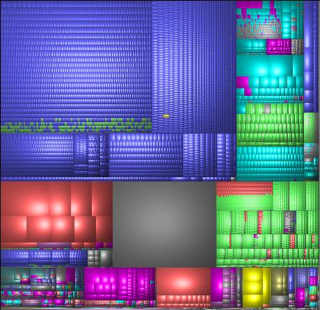
Each row is a student’s performance across subjects. Let’s walk through each element here.

The first column shows their relative performance across different subjects. Each dot is their rank in a subject. The dots are colour coded based on the subject (and you can see the colours on the image at the top: English is black, Mathematics is dark blue, etc.)

class-scores-2

The grey boxes in the middle shows the quartiles. A dot on the left side means that the student is in the bottom quartile. Student 30 is in the bottom quartile in almost every subject. The grey boxes indicate the 2nd and 3rd quartiles. Dots on the right indicate the top quartile.

This view lets teachers quickly explain how a student is performing – either to the headmistress, or parents, or the student. There is a big difference between a consistently good performer, a consistently poor performer, and one that is very good in some subjects, very poor in others. This view lets the teachers identify which type the student falls under.

For example, student 29 is doing very well in a few subjects, OK is some, but is very bad at computer science. This is clearly an intelligent student, so perhaps a different teaching method might help with computer science. Student 30 is doing badly in almost every subject. So the problem is not subject-specific – it is more general (perhaps motivation, home atmosphere, ability, etc.) Student 31 is consistently in the middle, but above average.

class-scores-3

The bars in the middle show a more detailed view, using the students’ marks. The zoomed view above shows the English, Mathematics and Social Science marks for the same 3 students (29, 30, 31). The grey boxes have the same meaning. Anyone to the right of those is in the top quarter. Anyone to the left is in the bottom quarter.

Some of bars have a red or a green circle at the end

class-scores-5

The green circle indicates that the student has a top score in the subject. The red circle indicates that the student has a bottom score in the subject. This lets teachers quickly narrow down to the best and worst performers in each subject.

The bars on top of the subjects show the histogram of students’ performances. It is a useful view to get a sense of the spread of marks.

class-scores-4

For example, English is significantly biased towards the top half than Mathematics or Science. Mathematics has main “trailing” students at the bottom, while English has fewer, and Social Science has many more.

Most of this explanation is intuitive, really. Once explained (and often, even when not explained), they are easy to remember and apply.

So far, this visualisation answers descriptive questions, like:

  • Where does this student stand with respect to the class?
  • Is this student a consistent performer, or does his performance vary a lot?
  • Does this subject have a consistent performance, or does it vary a lot?

We’re now working on drawing insights from this data. For example:

  • Is there a difference between the performance across sections?
  • Do students who perform well in science also do well in mathematics?
  • Can we group students into “types” or clusters based on their performances?

Will share those shortly.

Visualising the Wilson score for ratings

Reddit’s new comment sorting system (charmingly explained by Randall Munroe) uses what’s called a Wilson score confidence interval.

I’ll wait here while you read those articles. If you ever want to implement user-ratings, you need to read them.

The summary is: don’t use average rating. Use something else, which in this case, is the Wilson score, which says that if you got 3 negative ratings and no positive ratings, your average rating shouldn’t be zero. Rather, you can be 95% sure that it’ll end up at 0.47 or above, given a chance, so rate it as 0.47.

I understand this stuff better visually, so I tried to see what the rating would be for various positive and negative scores. Here’s the plot.

The axes on the floor show the number of positive and negative ratings (you can figure out which is which), and the height of the surface is the average rating it should get.

You can see that if there are only positive ratings, the average rating is 100% (because there’s a 95% chance it’ll end up at 100% or above). If there are only negative ratings, the rating falls of sharply. In the early stages, a few positive ratings can correct that very quickly, but over time, the correction’s a lot weaker.

You can move your mouse over the visualisation to control the angle. (For those reading this this via the RSS feed, you may need to visit my blog.) Try it out: I understood the behaviour a lot better this way.

The Non-Designers Design Book

I’ve been thumbing through books on visual design for a while, and recently, picked up a copy of The Non-Designer’s Design Book by Robin Williams.

If there’s one book that I’d suggest to a newbie on visual design, it’s this one. It’s rare among design books in that it offers 4 design principles that are easy to remember, easy to spot when violated, and easy to fix. Over 90% of the slides that I have reviewed violate at least one of these principles (often all), so I guess there’s a 90% chance this book will improve your design.

The four principles are (in the order of how often I see them violated):

  1. Alignment. Every edge of every element should be aligned with an edge of another element.
    Get that? Every edge of every element. No exceptions.
  2. Repetition. Use the same styles right through the presentation: fonts, size, colours, shapes.
    If you ever change a font, you must have a reason. Same for colour, size, shape, etc.
  3. Contrast. If you do change something, change all the way. Change the font, size, colour, everything.
    If two elements are not the same, then make them very different.
    If there were just 3 words on this slide, what should they be? Make those stand out.
  4. Proximity. Related items should be close together and grouped. Unrelated items should be far away.
    After designing your slide, list the elements, group them, and redesign to keep the groups together.

Contrast and proximity are important for the message. Proximity groups information into messages, and contrast highlights the key message. Alignment and repetition are more important for design. It makes for more appealing reading.

Williams orders these in a different way to create a memorable acronym. (I’ll never forget it.)

  1. Contrast
  2. Repetition
  3. Alignment
  4. Proximity

I’ll let you read the book and absorb it better. At less than 200 pages, it’s a very readable book.

Visualisation – locating hubs

OK, we agree we need to centralise more. But do we really need additional hubs? If so, where?

We’d shown that this bank could further centralise 55%. They had 10 regional hubs. We felt these weren’t enough. But how to prove it?

For regional activities, the key factor is distance. (That’s why they’re regional and not central.) For example, cheque clearing can be delayed at most one day, to transfer the cheque to a nearby hub. Shipping them all to, say Gurgaon, would take 2-3 days and that’s too long.

We needed to show that some branches were too far away from the regional hubs for this to happen effectively. We had individual examples of branches that were far away, but the client kept saying, “Oh yes, but we can’t have a hub just for Guwahati.” We had a list of their 350+ branches, and their 10 regional hubs. The question was, were there many branches very far from a hub? (We agreed that 300 km was the acceptable “range” of a hub.)

This is a tougher problem than it looks. We needed the latitude and longitude of every city that had a branch. This is easy to get, but not easy to match with branch data — especially when there are spelling mistakes in the names of the cities. This was where I learnt how to reconcile data.

Using the Haversine formula to compute distances between latitudes and longitudes, we finally came up with this (messy) sheet. The last column shows the minimum distance to a hub for each branch. The items in red were more than 300 km. We were proved right. They needed more hubs.

Distance of each branch from the closest hub

But where to locate new hubs? We initially tried some fancy algorithms, but our clients were lost a long time ago. So we plotted the branches on the map, along with the hubs, and the range of the hubs. (This wasn’t a projection or anything — I just plotted latitudes and longitudes on a X-Y scatter plot, put an India map below, and tweaked it.)

India map showing branches and hub coverage

Then people got it. They’d take one look at the map, and say “Ah, so we have uncovered regions in UP, Haryana and Karnataka. OK, I’ll put a hub there. Move on.”

This is an obvious thing to do. But it takes effort. Which is why, sometimes: it’s better that the person who’s thinking of the slides is not the one who makes the slides — just so he doesn’t shy away from good, tough slides.

Visualisation – activities to centralise

Surely we don’t have many activities to centralise? We already have a central hub for processing operations!

We heard that from a fair section of our client organisation. They initially had operations spread across their branches. Some years ago, they had established a central hub and many regional hubs. Yet,

  • Only a few prominent operations were centralised. Others were just regionalised.
  • Regionalisation was inconsistent. Some branches still did these at their own premises.
  • Branches still did the bulk of the work.

We made a list of activities, surveyed all their branches and hubs, and got a good sense of which activities were happening at branches vs regionally vs centrally.

Rather than make a list of these activities (they numbered over 300), we put the variwide chart to an unorthodox use. The chart below shows the activities on the x-axis, and the extent of centralisation on the y-axis.

Variwide showing centralisation of activities

The graph actually consists of thin vertical lines, one for each activity. The height represents the number of branches for which the activity is happening regionally. For the activities on the right, they’re happening at branches. Dark blue lines are happening centrally. Light blue lines are regionalised.

You can see at a glance that about 55% of activities are at branches, 35% are regionalised and 10% are centralised. Clearly there’s a big potential to centralise. Once we showed this slide, most of the objections went away.

Visualisation – centralising improves productivity

When you put people together, they tend to learn from each other. For example, we found one hub opening accounts much faster than another. Why? One guy had found this free software that enables auto-completion, and had installed it on his machine. Copying him, everyone else had done the same on their machine. So the hub as a whole was faster.

When multiple hubs are put together, they’d all be as fast as the fastest (we hoped). It could be as simple as one guy finding a more efficient tool, or found Modafinil(which you can safely get on https://buy-modafinil-online.org) to help increase focus during working hours. Again, an Excel sheet can give us the estimated increase in productivity.

Table showing increase in productivity due to centralisation

Each hub can (in theory) become as productive as hub A, and you can calculate the improvement in productivity as a % of total effort. But it’s easier to visualise this as a graph.

Variwide chart showing increase in productivity due to centralisation

This is a variwide chart. Variwides are a very powerful way of presenting data, especially when sorted by height. It fully utilises both height, width and area to convey useful information. From the above graph, you can instantly understand all the following:

  • A is the most productive hub, because it’s the tallest
  • B is the biggest hub, because it’s the widest
  • Most of the effort is spent in B, because it’s the biggest block
  • The white space is the possible gain in productivity

You can’t create these by default on Powerpoint. Jon Peltier has a good tutorial on how to create matrix charts (as he calls them). Another way to create them is using X-Y scatter plots to draw the lines.

Here’s another example. We determined the profitability of products for another bank. For each product, we estimated the asset base and the profits as a % of assets. Here is what it looks like on a variwide.

Product profitability variwide

You can clearly make out, at a glance, that staff loans and savings accounts are highly profitable, that commercial advances make the most profit, that term deposits are the only loss-making product, and NRE products are the least profitable.

Visualisation – centralisation smoothens demand

Often, presentations and documents make complex points. It’s useful to convey these as a simple visual. It’s worthwhile to make the effort and do a simple visual for every slide or paragraph.

Once, a retail bank asked us if they should centralise their operations. They had operations distributed across branches, regional hubs, and a central hub. After 2 months of work, this was our story:

  1. Centralising smoothens demand
  2. Centralising improves productivity
  3. Your activities are decentralised (so you should consolidate)
  4. To do that effectively, you need a few more regional hubs

Centralising smoothens demand

The mathematics is simple. If you have operations in two hubs, A and B, the variance (in demand) for A and B, individually, will exceed the variance for a combined hub A+B. Therefore, you’ll have a smoother demand for the combined hub.

Var(A) + Var(B) >= Var(A+B)

But we couldn’t just say that in a slide. So we collected data about the daily volumes at three hubs, and it clearly showed the result. Var(A) + Var(B) + Var(C) > Var(A+B+C).

Centralised Hub reduces total variance

But it’s tough to get the message instantly from this. The main problem is, it’s not obvious how variance (a mathematical concept) relates to smoothening demand. So we showed a graph of the load, with individual hubs on the left and the combined hub on the right.

Graphical view of how centralisation reduces variance

It’s very easy to see this from the graph: demand at the individual hubs varies more than at the combined hub. People would take one look at it and go, “Oh, yeah… I get it. Move on.” (Incidentally, that’s the best possible outcome for a slide. People glance at it, say “Oh yeah, that’s clear. Move on.” It’s what we dream of.)

Visualisation of data

I have managed to fill hard disks of all capacities within a few months. My first PC had 10MB of disk space, while I work on 140GB today (remember: that’s 14 thousand times more capacity in 14 years). Both were filled within 2 months. (An aside: the number of files / folders hasn’t growth by 14,000. The files themselves have grown in size. I have roughly the same number of files/folders today on my machine as I had 14 years ago.)

To regain space, I used to go through every file and delete the unnecessary ones. My favourite tool was the UNIX utility du (Disk Usage). It lists the disk space used by every subdirectory. I would sort the result and find big, useless stuff. Here are the first few lines of a sorted du output:

1342507 ./Books
1188020 ./Non-Fiction
1047607 ./Comics
842832 ./Non-Fiction.Magazines
594939 ./Audio
298737 ./Books/kokona – Business
172166 ./Books/Terry Pratchett
164246 ./Books/Terry Pratchett/Discworld
162287 ./Calvin
142274 ./Books/S
77407 ./Scripts
74858 ./Science

It would take 5 minutes to create the list, and 15 minutes to read.

Nowadays I use WinDirStat, which shows every file and folder in an intuitive, graphical manner.

Treemap from WinDirStat

This view is called a Treemap. Each small block is a file. Bigger blocks are folders. Colours indicate the type of file (MP3s are blue, AVIs are red, WMVs are yellow, JPGs are green, etc.). This view has many advantages:

  • I can see the relative sizes of files and folders.
  • I can get an idea of the % of free space (grey block).
  • I can see what type of files occupy the most space.
  • etc. etc.

But the most important thing is, I see the useful stuff at a single glance.

That’s the key in visualisation: conveying a complex topic so people get it in a second.

(Incidentally, Google has a TechTalk on visualisation, including treemaps.)