From Calvin & Hobbes to Photo Tagging: Excel's Unexpected Image Capability
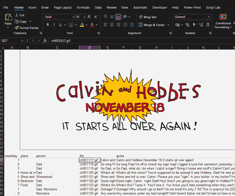
In Excel, using Visual Basic, you can change an image as you scroll. This makes it easy to look at each image and annotate it. This is how I transcribed every Calvin & Hobbes. I used this technique first when typing out the strips during my train rides from Bandra to Churchgate. I had an opportunity to re-apply it recently when we needed to tag hundreds of photographs based on a set of criteria. ...