Rule #3: Avoid manual labour (continued)
Reconciling data is where I spend most of my time on Excel. Say you have a list of branches by city from 2 banks. You want to know where both banks have branches. Excel doesn’t know that Kolkata is Calcutta. There are 500 cities, and you have 30 minutes.
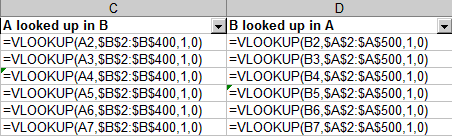
Use VLOOKUP for a start. If Bank A’s cities are in column A (say 2-500) and Bank B’s cities in column B (say 2-400), in C2 type VLOOKUP(A2, B$2:B$400, 1, 0) (read Excel help – all I’ll say is, don’t miss out the 0 at the end: otherwise you get approximate match, and that’s not good). Copy the formula to down to C500. Similarly, in D2 type VLOOKUP(B2, A$2:A$500, 1, 0). Copy the formula down to D400.
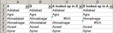
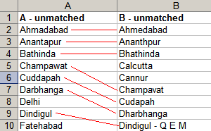
You’ll see the #N/A where there’s no match. #N/A in Column C means Bank A has a branch here, but Bank B does not. Column D has the converse. But we’re not done yet. There could be spelling mistakes. Using two VLOOKUPs simplifies that problem considerably. We just need to match the cities having #N/A on both lists to check for alternate spellings of cities – which is a lot less work! So prepare a separate list: unmatched cities from Bank A, and unmatched cities from Bank B. (See the section on removing unwanted rows to simplify this.)
Sort both the lists while remembering the original order. You’ll want to remember the original order often – so just add a column, number it sequentially (1,2,3… use Alt-E-I-S), and sort the city names along with the numbers. When you want to get back the original order, just sort by the numbers again. To avoid distraction, you can move or hide these numbers. Now, you have a sorted list of unmatched cities. Notice that you can visually match many of these cities. There’s nothing easier to search (visually) than a sorted list.
Finally, when you’ve mapped all your columns, the ones that are remaining are the ones where there is no overlap.
Comments
What I did was use the ‘Advanced Filter’ function in Excel and wrote a small VB program to list out the filtered results in a dialog box allowing user to select the relevant ones using ‘human’ intelligence.
The trick was in identifying a small enough part of the company’s name that would serve as a ‘signature’ and at the same time throw back as (few) relevant results. What worked best for me was the following: \