Dynamically sort data

This is a series on what Google Spreadsheets can do that Excel can’t.

To sort data, use the SORT function.

For example, if you have a list of products, their revenues and profits in A2:C9. Type SORT(A2:C9, 2, FALSE) in cell E2 to get the products sorted by the second column, revenues.

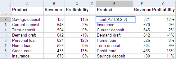
This is a dynamic list. If you change the revenues, the products are reordered automatically.

The first parameter to the SORT function is the data range you want to sort. The remaining parameters are optional. The second parameter is the column to sort by. By default, the data is sorted by the first column, in ascending order. In this example, we sorted by the 2nd column. The third parameter is FALSE for descending order, and TRUE for ascending order.

You can specify additional columns to sort by. Just add the second column number and the order, third column number and order, and so on.

For example, this formula sorts by the 2nd column (ascending), 4th column (descending) and 1st column (ascending):

=SORT(A1:D100, 2, TRUE, 4, FALSE, 1, TRUE)

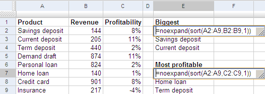
You can create a dashboard with multiple views. Say you wanted to show the above data, and also summarise the top 3 products by revenue and profitability. Go to cell E2, and type

=NOEXPAND(SORT(A1:A9, B2:B9, TRUE))

This sorts the products (A1:A9) using the revenues (B2:B9) in ascending order (TRUE or 1). This would show all 8 products. If you want to keep only the top 3, you need to put the NOEXPAND around the formula. Otherwise, even if you delete the 4th product, Google will put it back.

Now, delete all but the top 3 products. Similarly, in cell E7, type

=NOEXPAND(SORT(A1:A9, C2:C9, TRUE))

This sorts by profitability instead. That’s it! You have a dynamic list of the top 3 products by revenue and profitability.

Can I do that in Excel?

Excel doesn’t have a function to sort. You can sort a list in-place. That changes the order permanently. There’s no way of retaining the original order.

You could make a copy of the list and sort it. But the copy will not change when the original list changes.

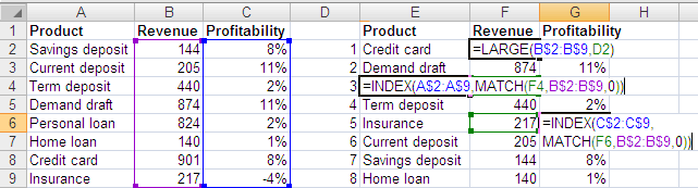
If the length of the list is fixed, and the values you want to sort by are unique, you could use the LARGE/SMALL, INDEX and MATCH functions to simulate this effect. First, type the numbers 1-8 in column D. Then type this formula in F2:

=LARGE(B$2:B$9,D2)

This will give you the largest revenue figure. Copy this down the column. This will show the largest revenue figures in descending order. Now, fill cells E2 downwards with the formula:

=INDEX(A$2:A$9,MATCH(F2,B$2:B$9,0))

The MATCH function finds the revenue in the first table, and the INDEX function looks up the corresponding product. You can use the same principle to get the profitability. However, this will not work if two products have the same revenue figure.