Excel tips

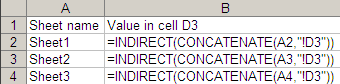
A corollary of Rule 3: Never type the same formula twice. Design the formula so that if you cut and paste it elsewhere, it works correctly. The $ symbol and the F4 key for cell references help in 90% of the cases. For complex requirements and large data, 5 functions come in handy: INDIRECT, OFFSET, ADDRESS, ROW and COLUMN. I once did a survey, and had data spread across 300 sheets (same format on all sheets). I needed cell D3 across all sheets in a column, to summarise the results. The image explains what I did. ...

Rule #3: Avoid manual labour (continued) Reconciling data is where I spend most of my time on Excel. Say you have a list of branches by city from 2 banks. You want to know where both banks have branches. Excel doesn’t know that Kolkata is Calcutta. There are 500 cities, and you have 30 minutes. Use VLOOKUP for a start. If Bank A’s cities are in column A (say 2-500) and Bank B’s cities in column B (say 2-400), in C2 type VLOOKUP(A2, B$2:B$400, 1, 0) (read Excel help – all I’ll say is, don’t miss out the 0 at the end: otherwise you get approximate match, and that’s not good). Copy the formula to down to C500. Similarly, in D2 type VLOOKUP(B2, A$2:A$500, 1, 0). Copy the formula down to D400. ...

Rule #3: Avoid manual labour. Use Excel to automate the task. I use Excel’s formulas to speed up repetitous tasks. These techniques are powerful, meaning, you can do a lot with a little, but can have unforeseen consequences. Excel can find and replace formulas. If you had hardcoded formulas and wanted to change =B1*3.14 to =B1*3.1416 across all rows, just find “*3.14” and replace it with “*3.1416”. Find and replace works in formulas. This is very powerful. You can use it to change the source (e.g. change the source from column B to C by finding “=B” and replacing with “=C”) or even the formula (find and replace “SUM(” with “SUBTOTAL(9,”). ...

Rule #2: Never type in data in Excel. You rarely spend time creating voluminous data. Usually, you’re just processing it (copying, transforming, whatever). Sometimes data is on a web page – typically tables. To copy such data, open the page in Internet Explorer and paste it in Excel. You won’t like the formatting. So copy the cells you just pasted, go to a different sheet, and Edit-Paste Special just the values (Alt-E-S-V-Enter). ...

I spend a lot of time building models on Excel. I have 4 rules that help me get things done fast. Never use the mouse. The keyboard is much faster. Never type in data. You can always import it. Avoid manual labour. Use Excel to automate the task. Make your data visually obvious. Let’s look at Rule #1: Never use the mouse. Using the keyboard can be 10 times faster than the mouse. It takes time to move one hand from the keyboard to the mouse, locate the item you want to click at, move the mouse there, adjust it finely so it’s pointing at the exact spot, and then click it. For example, to insert text without formatting, I’d just go Alt-E, S, enter. It takes half a second. It took me 5 seconds with a mouse. (I timed 10 continuous attempts in both cases.) ...