Excel – Avoid manual labour 3

A corollary of Rule 3: Never type the same formula twice. Design the formula so that if you cut and paste it elsewhere, it works correctly. The $ symbol and the F4 key for cell references help in 90% of the cases. For complex requirements and large data, 5 functions come in handy: INDIRECT, OFFSET, ADDRESS, ROW and COLUMN.

I once did a survey, and had data spread across 300 sheets (same format on all sheets). I needed cell D3 across all sheets in a column, to summarise the results. The image explains what I did.

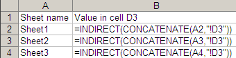
INDIRECT returns the value of a cell. INDIRECT(“Sheet2!D3″) is the value of cell D3 in Sheet2. And INDIRECT(CONCATENATE(A2,”!D3″)) will give you the value of cell D3 in whatever sheet A2 specifies! I created a list of sheet names in column A, and column B had “D3” in each of those sheets. In effect, INDIRECT can transpose sheets into columns.

Getting a list of sheet names on to a column is tough, however. If your sheets are sequentially numbered, this image shows a trick that may help.

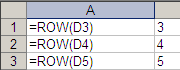
If you need multiple cells from a sheet, say D3:Z3, use the ADDRESS, ROW and COLUMN functions. ROW(D3) returns 3, and COLUMN(D3) returns 4 — the respective row and column. If you copy ROW(D3) to multiple rows, you will see ROW(D3), ROW(D4), ROW(D5), … which are 3, 4, 5 respectively. Similarly for COLUMN. It’s a useful way of linking values to position.

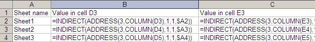
ADDRESS does the opposite. ADDRESS(ROW(D3),COLUMN(D3)) = ADDRESS(3,4) = “$D$3”. ADDRESS(3,4,1,1,”Sheet2″) returns “Sheet2!$D$3”. (See help for the ,1,1 in the middle, and just put it in always.) To cells D3:Z3 from all the sheets, copy the formula INDIRECT(ADDRESS(3,COLUMN(D3),1,1,$A2)) to the entire range. The INDIRECT, ADDRESS, ROW/COLUMN combination can slice contiguous data across sheets in any way you want.

Another useful function is OFFSET. OFFSET(D3,2,1) returns the value in cell E5. It shifts the reference D3 down by 2 rows and right by 1 column. OFFSET can be used instead of the INDIRECT and ADDRESS when multiple sheets are not involved. OFFSET can also return a range. OFFSET(D3,0,0,2,2) returns the range D3:E4, which is the 2×2 range starting from 0,0. So SUM(OFFSET(D3,0,0,2,2)) is the same as SUM(D3:E4). With OFFSET, you can specify a range with variable position and variable size (which you can’t with $ references).

Once, we were modelling a leasing company’s accounts. (Warning: this is a complex example.) We knew the volume of loans they would disburse over the next 3 years. The monthly interest rate is, say, 1%. What would be their interest income every month? Well, it’s not just 1% of what they’ve lent out. Customers pay back in equal monthly installments (EMIs). The EMI includes the principal and the interest. Initially, the EMI has a large interest component and very little principal, because there’s a lot left to repay. Towards the end, the balance dies down and so does the interest; it’s mainly the balance principal that’s being repaid. The interest income is not the same every month even for a single lease.

The calculation is conceptually simple. The IPMT function tells you the monthly interest each month. Let’s say all leases are for 36 months. So, to calculate the March interest income, take the January disbursals and multiply it by the third month interest component: IPMT(1%,3,36,-1). Take the Feb disbursals and multiply it by IPMT(1%,2,36,-1). Take the March disbursals and multiply it by IPMT(1%,1,36,-1). And add them up. For April, you’d add 4 terms. And so on. Mathematicians call this a convolution. It’s like a SUMPRODUCT of a series with another series in reverse.

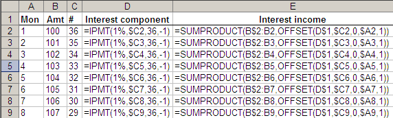
Cell E4 on the image alongside does exactly that for month 3 (March). There are 5 columns:
A: Month
B: Amount disbursed that month
C: Months in reverse
D: Interest component for month in reverse
E: Interest income for month
E4 is the sumproduct of B2 to B4 (the Jan, Feb and March disbursals) with something else — an OFFSET. The offset says, from D1, move down C4 (34) rows and select A4 (3) cells further down. This has the interest components for the first, second and third months in reverse. So, the disbursal for Jan is multiplied with the 3rd month’s interest, Feb with the 2nd month’s interest, and Mar with the 1st month’s interest. That’s exactly what we wanted.

It may look complex. But remember: you have to type this complex formula only once, not 36 times. (And in my case, I had 18 product types.) Also, you’re less likely to make typing errors when cutting and pasting. So this saves you debugging time as well.