I used this technique first when typing out the strips during my train rides from Bandra to Churchgate. I had an opportunity to re-apply it recently when we needed to tag hundreds of photographs based on a set of criteria.
Here’s how you can do this. Note: This works only on Windows.
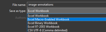
STEP 1: Create a new Excel workbook and save it as an Excel macro-enabled workbook. (Note: When opening it again, you need to enable macros)
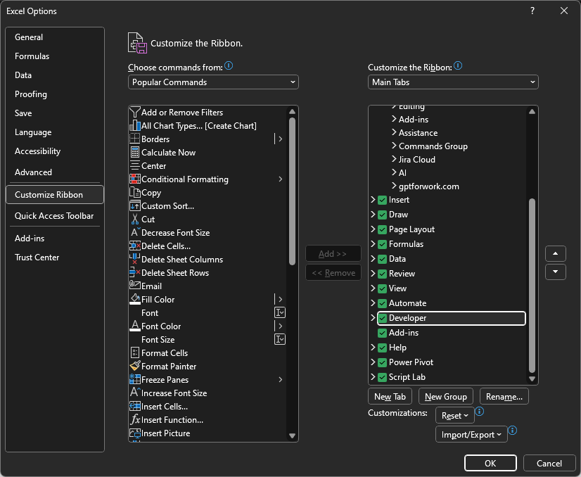
STEP 2: Open File > Options (Alt-F-T), go to Customize Ribbon. Under “Customize the Ribbon”, enable the “Developer” menu.
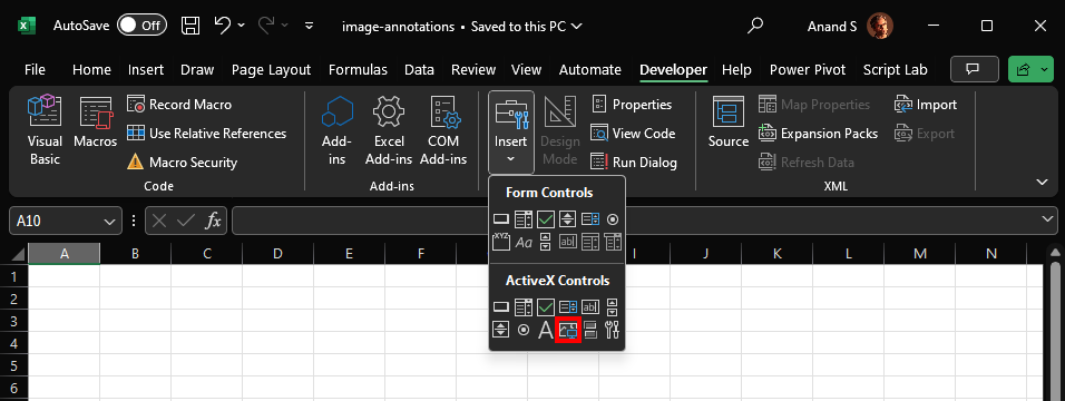
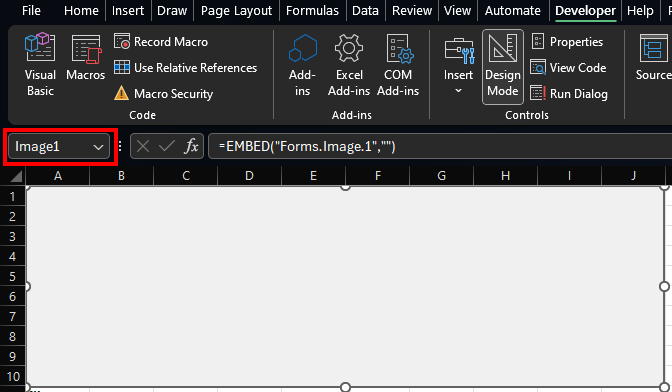
STEP 3: In Developer > Insert > ActiveX Controls, select Image and draw a rectangle from A1 to J10. (Resize it later.)
STEP 4: By default, this will be called Image1. In any case, note down the name from the Name box on the top left.
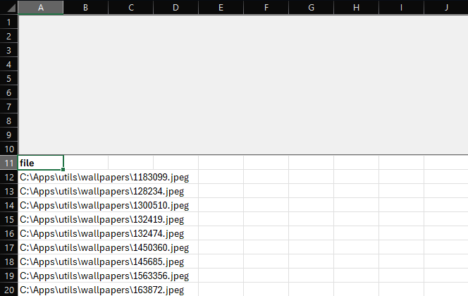
STEP 5: In cells A11 onwards, add paths to file names.
STEP 6: Click Developer > Visual Basic (Alt-F11), go to ThisWorkbook, and paste this code:
Option Explicit

Private Sub Workbook_SheetSelectionChange(ByVal Sh As Object, ByVal Target As Excel.Range)
    Dim img As String
    img = Sh.Cells(Target.Row, 1).Value
    If (img <> "" And img <> "file") Then ActiveSheet.Image1.Picture = LoadPicture(img)
End Sub
Replace ActiveSheet.Image1 with ActiveSheet.(whatever) based on your image name in Step 4.
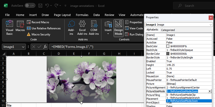
STEP 7: Select Developer > Design Mode. Click on Image1. Then select Developer > Properties. In this panel, under PictureSizeMode, choose 3 - fmPictureSizeModeZoom to fit the picture.
Now scroll through the rows. The images will change.
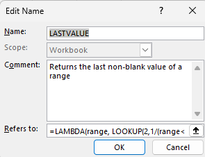
So, I followed the instructions to create a function in the Name Manager (Ctrl+F3)
… and simply fill in =LASTVALUE(H6:S6) and the like in the “Skills Index” cell.
The LOOKUP formula is confusing. My aim is to confuse our team less. But I wonder if they’ll start Google-ing for this LASTVALUE formula no one ever heard of, and get more confused 🤔.
Creating motion charts in Excel is a simple four-step process.
Get the data in a tabular format with the columns [date, item, x, y, size]
Make a “today” cell, and create a lookup table for “today”
Make a bubble chart with that lookup table
Add a scroll bar and a play button linked to the “today” cell
For the impatient, here’s a motion chart spreadsheet that you can tailor to your needs. For the patient and the puzzled, here’s a quick introduction to bubble and motion charts.
What is a bubble chart?
A bubble chart is a way of capturing 3 dimensions. For example, the chart below could be the birth, literacy rate and population of countries (X-axis, Y-axis and size). Or the growth, margin and market cap of companies.
It lets you compare three dimensions at a glance. The size dimension is a different from the X and Y axes, though. It’s not easy to compare differences in size. And the eye tends to focus on the big objects. So usually, size is used highlight important things, and the X and Y axes used to measure the performance of these things.
If I were to summarise bubble charts in a sentence, it would be: bubble charts show the performance of important things (in two dimensions). (In contrast, Variwide charts show the same on one dimension.)
Say you’re a services firm. You want to track the productivity of your most expensive groups (“the important things”). Productivity is measured by 2 parameters: utilisation and margin. The bubble chart would then have the expense of each group as the size, and its utilisation and contribution as the X and Y axes.
What is a motion chart?
Motion charts are animated bubble charts. They track the performance of important things over time (in two dimensions). This is chart with 4 dimensions. But not all data with 4 dimensions can be plotted as a motion chart. One dimension has to be time, and another has to be linked to the importance of the item.
Motion charts were pioneered by Hans Rosling and his TED Talk shows you the true power of motion charts.
How do I create these charts?
Use the Motion Chart Gadget to display any of your data on a web page. Or use Google Spreadsheets if you need to see the chart on a spreadsheet: motion charts are built in.
If you or your viewer don’t have access to these, and you want to use Excel, here’s how.
1. Get the data in a tabular format
Get the data in the format below. You need the X, Y and size for each thing, for each date.
Date
Thing
X
Y
Size
08/02/2009
A
64%
11%
1
08/02/2009
B
14%
33%
2
08/02/2009
C
78%
55%
3
08/02/2009
D
57%
73%
4
08/02/2009
E
39%
32%
5
08/02/2009
F
40%
81%
6
09/02/2009
A
64%
12%
1
09/02/2009
B
14%
33%
2
09/02/2009
C
78%
56%
3
09/02/2009
D
57%
73%
4
09/02/2009
E
39%
32%
5
09/02/2009
F
40%
81%
6
…
…
…
…
..
To make life (and lookups) easier, add a column called “Key” which concatenates the date and the things. Typing “=A2&B2” will concatenate cells A2 and B2. (Red cells use formulas.)
Date
Thing
Key
X
Y
Size
08/02/2009
A
39852A
64%
11%
1
08/02/2009
B
39852B
14%
33%
2
08/02/2009
C
39852C
78%
55%
3
08/02/2009
D
39852D
57%
73%
4
…
…
…
…
…
…
2. Make a “today” cell, and create a lookup table for “today”
Create a cell called “Offset” and type in 0 as its value. Add another cell called Today whose value is the start date (08/02/2009 in this case) plus the offset (0 in this case)
Offset
0
(Just type 0)
Today
08/02/2009
Use a formula: =STARTDATE + OFFSET
Now, if you change the offset from 0 to 1, “Today” changes to 09/02/2009. By changing just this one cell, we can create a table that holds the bubble chart details for that day, like below.
This is a simple Insert – Chart. Go through the chart types and select bubble. Play around with the data selection until you get the X, Y and Size columns right.
4. Add a scroll bar and a play button linked to the “today” cell
Now for the magic. Add a scroll bar below the chart. Excel 2007 users: Go to Developer – Insert and add a scroll bar. Excel 2003 users: Go to View – Toolbars – Control Toolbox and add a scroll bar
Right click on the scroll bar, go to Format Control… and link the scroll bar to the “Offset” cell. Now, as you move the scroll bar, the value in the offset cell will change to reflect it. So the “today” cell will change too. So will the lookup table. And so will the chart.
Next, create a button called “Play” and edit its code. Excel 2007 users: Right click the button, go to Developer – View Code. Excel 2003 users: Right click the button and select View Code.
Type in the following code for the button’s click event:
DeclareSub Sleep Lib "kernel32" (ByVal dwMilliseconds AsLong)
Sub Button1_Click()
Dim i AsIntegerFor i = 0 To 40: ' Replace 40 with your range
Range("J1").Value = i ' Replace J1 with your offset cell
Application.Calculate
Sleep (100)
NextEndSub
Declare Sub Sleep Lib "kernel32" (ByVal dwMilliseconds As Long)

Sub Button1_Click()
    Dim i As Integer
    For i = 0 To 40:            ' Replace 40 with your range
        Range("J1").Value = i   ' Replace J1 with your offset cell
        Application.Calculate
        Sleep (100)
    Next
End Sub
Now clicking on the Play button will give you this glorious motion chart in Excel:
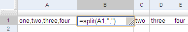
SPLIT(string, delimiter) splits a string using a delimiter. So if you have "one,two,three,four" in cell A1, you could split that into 4 cells using =SPLIT(A1,",")
That’s similar to Data > Text to Columns, except that if the original data changed, Text to Columns does not revise the output. SPLIT can give you dynamic text-to-columns. This is pretty useful when processing text data, in three ways:
You retain the original data
You don’t need to re-apply Text to Columns. Extending the formula will work (and that’s quicker)
It’s dynamic. If the data changes, your split changes
Since SPLIT returns an array, you can do a bunch of useful things with it.
=COUNTA(SPLIT(A1," ")) gives you the number of words in a string
=SUM(SPLIT(A1,",")) sums up a comma separated list. "1,2,3,4" is added up to 10.
=ARRAYFORMULA(SUM(LEN(SPLIT(A1,",")))) sums up the word lengths. So "one,two,three,four" splits into 4 words of length 3,3,5,4 each, which adds up to 15.
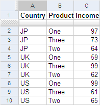
The ability to join and split also lets you sort by multiple keys. For example, say you had income by country and product. You want to show it sorted by Country & Product. You also want to show it by Product & Country.
So first take the data sorted by Country and Product.
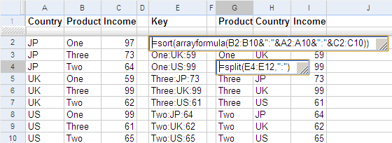
Now, in column E, create a key that’s sorted by Product and then by Income. Type
=SORT(ARRAYFORMULA(B2:B10&":"&A2:A10&":"&C2:C10))
… in cell E2. That will give you all the data in one cell, sorted by Product and then by Country. Now, just split the data, as shown here.
Note: You could have done the whole thing using one formula:
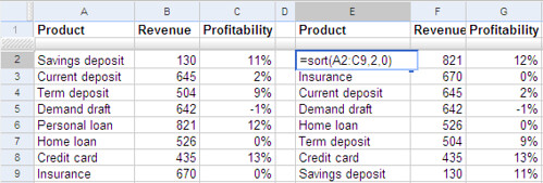
For example, if you have a list of products, their revenues and profits in A2:C9. Type SORT(A2:C9, 2, FALSE) in cell E2 to get the products sorted by the second column, revenues.
This is a dynamic list. If you change the revenues, the products are reordered automatically.
The first parameter to the SORT function is the data range you want to sort. The remaining parameters are optional. The second parameter is the column to sort by. By default, the data is sorted by the first column, in ascending order. In this example, we sorted by the 2nd column. The third parameter is FALSE for descending order, and TRUE for ascending order.
You can specify additional columns to sort by. Just add the second column number and the order, third column number and order, and so on.
For example, this formula sorts by the 2nd column (ascending), 4th column (descending) and 1st column (ascending):
=SORT(A1:D100, 2, TRUE, 4, FALSE, 1, TRUE)
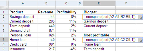
You can create a dashboard with multiple views. Say you wanted to show the above data, and also summarise the top 3 products by revenue and profitability. Go to cell E2, and type
=NOEXPAND(SORT(A1:A9, B2:B9, TRUE))
This sorts the products (A1:A9) using the revenues (B2:B9) in ascending order (TRUE or 1). This would show all 8 products. If you want to keep only the top 3, you need to put the NOEXPAND around the formula. Otherwise, even if you delete the 4th product, Google will put it back.
Now, delete all but the top 3 products. Similarly, in cell E7, type
=NOEXPAND(SORT(A1:A9, C2:C9, TRUE))
This sorts by profitability instead. That’s it! You have a dynamic list of the top 3 products by revenue and profitability.
Can I do that in Excel?
Excel doesn’t have a function to sort. You can sort a list in-place. That changes the order permanently. There’s no way of retaining the original order.
You could make a copy of the list and sort it. But the copy will not change when the original list changes.
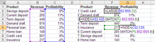
If the length of the list is fixed, and the values you want to sort by are unique, you could use the LARGE/SMALL, INDEX and MATCH functions to simulate this effect. First, type the numbers 1-8 in column D. Then type this formula in F2:
=LARGE(B$2:B$9,D2)
This will give you the largest revenue figure. Copy this down the column. This will show the largest revenue figures in descending order. Now, fill cells E2 downwards with the formula:
=INDEX(A$2:A$9,MATCH(F2,B$2:B$9,0))
The MATCH function finds the revenue in the first table, and the INDEX function looks up the corresponding product. You can use the same principle to get the profitability. However, this will not work if two products have the same revenue figure.
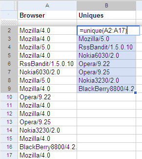
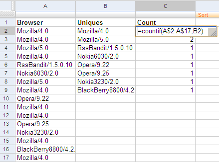
For example, if you have a list of browsers in column A, type =UNIQUE(A1:A17) at cell B1 to get a unique list of browsers. This is a dynamic list. If you change the list of browsers, the unique list gets updated automatically.
You can use UNIQUE to create a dynamic pivot table. Quite often, you end up creating a pivot table simply to summarise by one column. The main purpose the pivot table serves is in getting a list of unique values on that column. Plus, it’s a bit heavy on the UI. And every time the data changes, you need to refresh the pivot. But with the UNIQUE function, you can get a dynamic list of unique values, and you can use the COUNTIF and SUMIF function next to each value. Here is an example showing the frequency table of the browsers shown earlier. Column C does a COUNTIF of the unique values on the original list.
You can also use UNIQUE as the input to another formula:
=COUNT(UNIQUE(LIST)) counts the number of unique values
=COUNT(LIST)-COUNT(UNIQUE(LIST)) gives the number of duplicates
=INDEX(UNIQUE(LIST),3) gives you the third unique value
=LARGE(UNIQUE(LIST),3) gives you the third largest unique value
… and so on.
Can I do that in Excel?
You can, but not easily. There are two approaches, but each has its limitations.
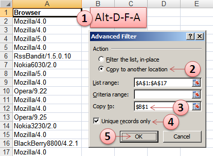
A. Use Advanced Filters: easy but static
Create an advanced filter on column A (Alt-D-F-A)
Select Copy to another location
Click in the Copy to box, and then click the cell B1
Select Unique records only
Click OK
But the list of unique values that you get here is static. If you changed one of the values, the list of unique values does not change.
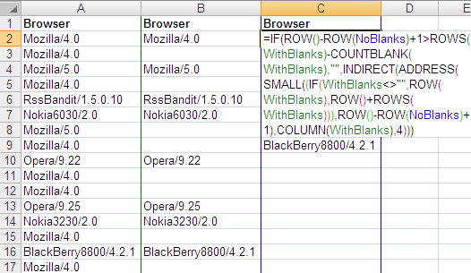
B. Use a complex formulae that are dynamic
First, blank out the duplicates by typing this formula:
=IF(COUNTIF(A$1:A1,A1)=1,A1,"")
adjacent to the first cell (into B1), and dragging it all the way down (to B17).
Now, create a named range (Alt-I-N-D) for these cells (B1:B17) called WithBlanks and another named range called NoBlanks for the cells one column to the right (C1:C17).
On the first cell of NoBlanks (C1), type this formula:
Press Ctrl-Shift-Enter rather than Enter, because it’s an array formula. Now drag this all the way down (to C17).
The list in column C is dynamic. If you change a cell in column A, column C is updated. But the formula can only handle one column. Google Spreadsheets’ UNIQUE function works with any number of columns. If you had data in the range A1:D100 and wanted the unique rows, UNIQUE(A1:D100) gets that for you.
Note: I’m staying away from user defined functions. You could, of course, create a UNIQUE function in Excel using Visual Basic. In fact, you should!
Yes. Google has a gadget called MotionChart that lets you do this.
Now, you could put this up on your web page, but that’s not quite useful when presenting to a client. (It is shocking, but there are many practical problems getting an Internet connection at a client site. The room doesn’t have a connection. The cable isn’t long enough. You can’t access the LAN. Their proxy requires authentication. The connection is too slow. Whatever.)
So you need this in Excel. Let me explain a variant of the technique I described earlier.
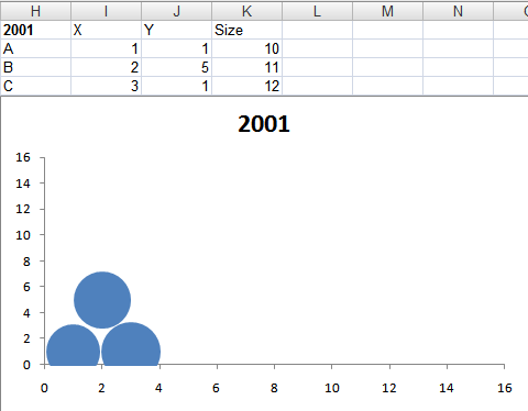
Let’s start by creating a simple bubble chart.
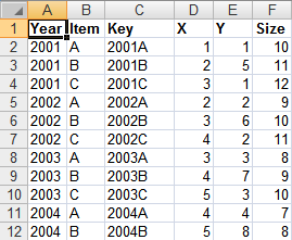
For each item in a bubble chart, you need 3 pieces of data: the X-axis, Y-axis and size. This graph shows three items A, B and C in one year: 2001. To animate this, you need data for more years, so let’s create that.
The first 3 rows contain the same data as before, except that I’ve added a "Year" column and a "Key" column (which is just a concatenation of the Year and the Item). The data now goes on for many more years.
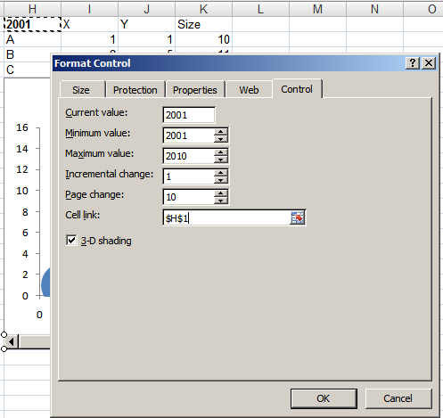
Now we need to create a scroll bar that can be used to change the year. So add a scroll bar below the bubble chart…
… and right click the scroll bar and go to Format Control. Now, select the cell link to some cell ($H$1 in this case). Now, if you move the scroll bar, the cell value will change.
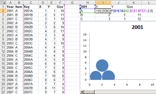
All you need to do is to now change the source data for the chart based on the year. From the table on the left, VLOOKUP the year + item, and put this into the table on the right. When the year in the cell H1 changes, the data updates itself. So now, as you move the scroll bar, cell H1 changes, then so does the data and hence the graph.
I’d written earlier about Web lookup in Excel. I showed an example how you could create a movie wishlist that showed the links to the torrents from Mininova.
=importData(“URL of CSV or TSV file”). Imports a comma-separated or tab-separated file.
=importFeed(URL).vLets you import any Atom or RSS feed.
=importHtml(URL, “list” | “table”, index). Imports a table or list from any web page.
=importXML(“URL”,”query”). Imports anything from any web page using XPath.
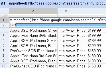
Firstly, you can see straight off why it’s easy to view RSS feeds in Google Spreadsheets. Just use the importFeed function straight away. So, for example, if I wanted to track all 8GB iPods on Google Base, I can import its feed in Google Spreadsheets.
This automatically creates a list of the latest 8GB iPods.
Incidentally, the “Price” column doesn’t appear automatically. It’s a part of the description. But it’s quite easy to get the price using the standard Excel functions. Let’s say the description is in cell C1. =MID(C1, FIND("Price", C1), 20) gets you the 20 characters starting from “Price”. Then you can sort and play around as usual.
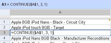
The other powerful thing about Google Spreadsheets is the CONTINUE function. The importFeed function creates a multi-dimensional array. You can extract any cell from the array (for example, row 3, column 2 from cell C1) using CONTINUE(C1, 3, 2). So you can just pick up the title and description, or only alternate rows, or put all rows and columns in a single column — whatever.
The most versatile of the import functions is the importXML function. It lets you import any URL (including an RSS feed), filtering only the XPath you need. As I mentioned earlier, you can scrape any site using XPath.
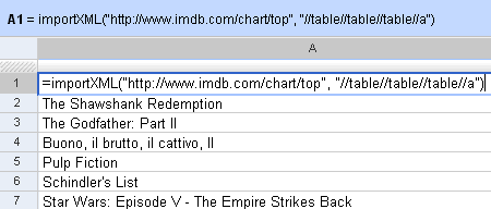
For example, =importXML("http://www.imdb.com/chart/top", "//table//table//table//a") imports the top 250 movies from the IMDb Top 250. the second parameter says, get all links (a) inside a table inside a table inside a table. This populates a list with the entire Top 250.
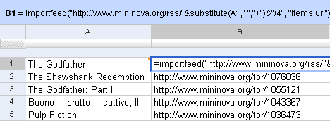
Now, against each of these, we could get a feed of Mininova’s torrents. Mininova’s RSS URL is http://www.mininova.org/rss/search_string. So, in cell B1, I can get a torrent for the cell A1 (The Godfather) using the importFeed function. (Note: you need to replace spaces with a + symbol. These functions don’t like invalid URLs.).
Just copy this formula down to get a torrent against each of the IMDb Top 250 movies!
Now, that’s still not the best of it. You can extract this file as an RSS feed! Google lets you publish your sheets as HTML, PDF, Text, XLS, etc. and RSS and Atom are included as well. Here’s the RSS feed for my sheet above.
Think about it. We now have an application that sucks in data from a web page, does a web-based vlookup on another service, and returns the results as an RSS feed!
There are only two catches to this. The first is that Google has restricted us to 50 import functions per sheet. So you can’t really have the IMDb Top 250 populated here — only the top 49. The second is that the spreadsheet updates only when you open it again. So it’s not really a dynamically updating feed. You need to open the spreadsheet to refresh it.
But if you really wanted these things, there’s always Yahoo! Pipes.
The technique of Web lookups in Excel I described yesterday is very versatile. I will be running through some of the practical uses it can be put to over the next few days
URL of the XML feed to read Search XPath list string (separated by spaces)
This function can be used to extract information out of any XML file on the Web and get it out as a table. For example, if you wanted to watch the Top 10 movies on the IMDb Top 250, and were looking for torrents, an RSS feed is available from mininova. The URL http://www.mininova.org/rss/movie_name/4 gives you an RSS file matching all movies with “movie_name”. From this, we need to extract the <item><title> and <item><link> elements. That’s represented by “//item title link” on my search string.
The formula becomes XPath2( "http://www.mininova.org/rss/"&A2&"/4", "//item title link"). The result is a 2-dimensional array returning individual items in rows, and the columns are title and link. Pulling it all together, you can get the sheet above.
All of this could be done using a command-line program. Excel has one huge advantage though. It’s one of the most powerful user-interfaces. Increasingly, I’m beginning to rely on just two user interfaces for almost any task. One is the browser, and the other is Excel. With Excel, I could have a sheet that has my movie wishlist (which changes often), and add check to see if the torrent exists. Every time I add a bunch of movies to the wishlist, it’s just a matter of copying the formula down. No need to visit a torrent search engine and typing each movie in, one by one.
Another example. Someone suggests 10 movies to watch. I’d rather watch the ones with a higher IMDb rating. Again, enter the Web lookup. Type in the movie names. Use a function like this to look up the rating on IMDb, and sort by the rating.