This is a series on what Google Spreadsheets can do that Excel can’t
To get a list of unique values from a list, use the UNIQUE function on Google Spreadsheets.
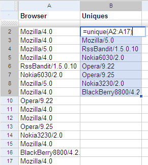
For example, if you have a list of browsers in column A, type =UNIQUE(A1:A17) at cell B1 to get a unique list of browsers. This is a dynamic list. If you change the list of browsers, the unique list gets updated automatically.
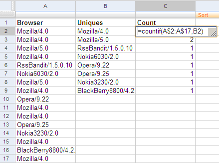
You can use UNIQUE to create a dynamic pivot table. Quite often, you end up creating a pivot table simply to summarise by one column. The main purpose the pivot table serves is in getting a list of unique values on that column. Plus, it’s a bit heavy on the UI. And every time the data changes, you need to refresh the pivot. But with the UNIQUE function, you can get a dynamic list of unique values, and you can use the COUNTIF and SUMIF function next to each value. Here is an example showing the frequency table of the browsers shown earlier. Column C does a COUNTIF of the unique values on the original list.
You can also use UNIQUE as the input to another formula:
=COUNT(UNIQUE(LIST)) counts the number of unique values
=COUNT(LIST)-COUNT(UNIQUE(LIST)) gives the number of duplicates
=INDEX(UNIQUE(LIST),3) gives you the third unique value
=LARGE(UNIQUE(LIST),3) gives you the third largest unique value
… and so on.
Can I do that in Excel?
You can, but not easily. There are two approaches, but each has its limitations.
A. Use Advanced Filters: easy but static
- Create an advanced filter on column A (Alt-D-F-A)
- Select Copy to another location
- Click in the Copy to box, and then click the cell B1
- Select Unique records only
- Click OK
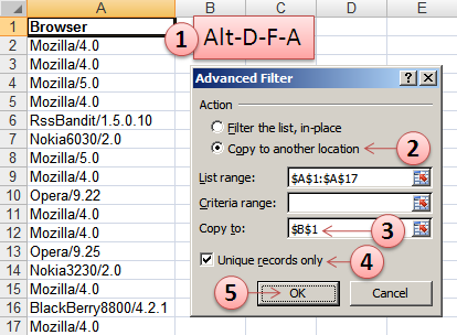
But the list of unique values that you get here is static. If you changed one of the values, the list of unique values does not change.
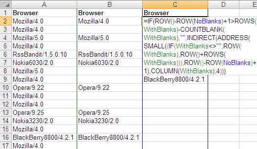
B. Use a complex formulae that are dynamic
First, blank out the duplicates by typing this formula:
=IF(COUNTIF(A$1:A1,A1)=1,A1,"")
adjacent to the first cell (into B1), and dragging it all the way down (to B17).
Now, create a named range (Alt-I-N-D) for these cells (B1:B17) called WithBlanks and another named range called NoBlanks for the cells one column to the right (C1:C17).
On the first cell of NoBlanks (C1), type this formula:
=IF(ROW()-ROW(NoBlanks)+1>ROWS(WithBlanks)-COUNTBLANK(WithBlanks),"",
    INDIRECT(ADDRESS(SMALL((IF(WithBlanks<>"",ROW(WithBlanks),ROW()+
    ROWS(WithBlanks))),ROW()-ROW(NoBlanks)+1),COLUMN(WithBlanks),4)))
Press Ctrl-Shift-Enter rather than Enter, because it’s an array formula. Now drag this all the way down (to C17).
The list in column C is dynamic. If you change a cell in column A, column C is updated. But the formula can only handle one column. Google Spreadsheets’ UNIQUE function works with any number of columns. If you had data in the range A1:D100 and wanted the unique rows, UNIQUE(A1:D100) gets that for you.
Note: I’m staying away from user defined functions. You could, of course, create a UNIQUE function in Excel using Visual Basic. In fact, you should!
Great entry. I love your site. It is perfect for advanced users.
Let’s hope Google’s pressure will force some innovation at excel.
What about Data/Consolidate from menu?